1 预备知识
1 数据操作
本节介绍在深度学习中的数组: 张量 (tensor). 它类似 numpy 的 ndarray, 但是支持 GPU 加速计算、自动微分.
1.1 入门
以 PyTorch 为例.
#导入PyTorch
import torch

x = torch.arange(12)
#tensor([0, 1, 2, 3, 4, 5, 6, 7, 8, 9, 10, 11])

#张量的尺寸
x.shape # torch.Size([12])

#张量中总元素的个数
x.numel() # 12
修改张量尺寸:
X = x.reshape(3, 4)
'''
tensor([[0, 1, 2, 3],
        [4, 5, 6, 7],
        [8, 9, 10, 11]])
'''
Y = x.reshape(3, 2, 2)
'''
tensor([[0, 1],
        [2, 3]],

       [[4, 5],
        [6, 7]],

       [[8, 9],
        [10, 11]])
'''
这里
reshape((3, 4))效果是等同的
如果只指定行或者列, 然后自动计算另一个维度, 可以直接填入-1:
x.reshape(-1, 4) #指定四列
x.reshape(3, -1) #指定三行
全零: 输入一个 tuple (同样等效于 torch.zeros(2, 3, 4))
torch.zeros((2, 3, 4))
'''
tensor([[[0., 0., 0., 0.],
         [0., 0., 0., 0.],
         [0., 0., 0., 0.]],

        [[0., 0., 0., 0.],
         [0., 0., 0., 0.],
         [0., 0., 0., 0.]]])
'''
类似地有 torch.ones((2, 3, 4))
逐元素从概率分布取值:
torch.randn(3, 4) #每个元素从N(0,1)正态分布取值
从 Python 列表转换:
torch.tensor([[2, 1, 4, 3], [1, 2, 3, 4], [4, 3, 2, 1]])
1.2 运算符
对两个 tensor 对象 x, y, 可以用 x+y, x-y, x*y, x/y, x**y 生成新的 tensor, 其中的元素进行逐元素运算.
对每个元素添加指数:
torch.exp(x)
多个 tensor 的连结 (concatenate):
X = torch.arange(12).reshape(3, 4)
Y = torch.tensor([2, 1, 4, 3], [1, 2, 3, 4], [4, 3, 2, 1])
torch.cat((X, Y), dim=0) # 按行拼接
torch.cat((X, Y), dim=1) # 按列拼接
'''
tensor([[ 0.,  1.,  2.,  3.],
        [ 4.,  5.,  6.,  7.],
        [ 8.,  9., 10., 11.],
        [ 2.,  1.,  4.,  3.],
        [ 1.,  2.,  3.,  4.],
        [ 4.,  3.,  2.,  1.]])
tensor([[ 0.,  1.,  2.,  3.,  2.,  1.,  4.,  3.],
        [ 4.,  5.,  6.,  7.,  1.,  2.,  3.,  4.],
        [ 8.,  9., 10., 11.,  4.,  3.,  2.,  1.]])
'''
构建 Bool 型张量: (需要尺寸一致)
X == Y
'''
tensor([[False,  True, False,  True],
        [False, False, False, False],
        [False, False, False, False]])
对所有元素求和: 得到单元素张量(并非 float!)
X.sum() #tensor(66.)

#可以求所有行的元素:
X.sum(axis=0)

#非降维求和: 求和后保持轴的数量不变
X.sum(axis=1, keepdims=True)
- 类似地,
mean,sum也可以使用axis来对指定轴进行运算.- 在 tensor 中, 维数特指轴的数量; 在向量中, 维数指元素个数.
点积: 按照
X = torch.ndarray([0, 1, 2, 3])
y = torch.ones(4)
torch.dot(x, y) # tensor(6.)
#这等价于torch.sum(x * y)
矩阵、向量:
torch.mv(A, y) #矩阵、向量
torch.mm(A, B) #矩阵、矩阵
范数:
torch.norm(u) #L2范数
torch.abs(u).sum() #L1范数
1.3 广播机制
广播机制用于自动为两个尺寸不同的张量填充尺寸, 以进行运算
a = torch.arange(3).reshape(3, 1)
b = torch.arange(2).reshape(1, 2)
a + b
#a变成: tensor([[0, 0], [1, 1], [2, 2]])
#b变成: tensor([[0, 1], [0, 1], [0, 1]])
#a+b: tensor([[0, 1], [1, 2], [2, 3]])
1.4 索引 切片
索引、切片和 Python 数组一致:
X[-1], X[1:3]

#修改指定元素
X[1, 2] = 9
X[0:2, :] = 12 #0、1两行的所有列的值变为12
1.5 内存
在 PyTorch 中, 如果我们执行 Y = Y + X, 则 Y 的内存发生了改变. 为了改变这一点, 需要原地操作: 使用 Y += X, 或者切片操作 Y[:] = X + Y.
1.6 转换为其他 Python 对象
A = X.numpy() #将torch.Tensor变为numpy.ndarray
B = torch.tensor(A) #将numpy.ndarray变为torch.Tensor
大小为一的张量转换为标量:
a = torch.tensor([3,5])
a.item(), float(a), int(a) #3.5, 3.5, 3
2 微积分
- 导数
. - 偏导数:
. - 梯度:
. - 链式法则:
.
一般地,有变量 , 每个 都有 , 因此 是 的函数, 则
3 自动微分
3.1 一个简单的例子
PyTorch 可以自动计算梯度
x = torch.arange(4.0)
x.requires_grad_(True) #等价于x = torch.arange(4., requires_grad=True)
x.grad #当前的值是默认值None

y = 2 * torch.dot(x, x) #tensor(28., grad_fn=<MulBackward0>)
y.backward()
x.grad #此时y'=4x, 因此tensor([0., 4., 8., 12.])
x.grad == 4*x #tensor([True, True, True, True])
现在计算另一个函数
x.grad.zero_() #默认情况下梯度会累积, 因此需要清除
y = x.sum()
y.backward()
x.grad #tensor([1., 1., 1., 1.])
3.2 非标量变量的反向传播
当
x.grad.zero_()
y = x * x
y.sum().backward() #y.backward(torch.ones(len(x)))
#(x_1^2+...+x_n^2)'=2(x_1+...+x_n)
x.grad #tensor([0., 2., 4., 6.])
3.3 分离计算
有时候我们希望将某些计算放在计算图之外. 例如
为此, 分离
x.grad.zero_()
y = x * x
u = y.detach()
z = u * x

z.sum().backward()
x.grad == u #tensor([True, True, True, True])

x.grad.zero_()
y.sum().backward()
x.grad == 2 * x #tensor([True, True, True, True])
Python 控制流的梯度计算
def f(a):
    b = a * 2
    while b.norm() < 1000:
        b = b * 2
    if b.sum() > 0:
        c = b
    else:
        c = 100 * b
    return c

a = torch.randn(size=(), requires_grad=True)
d = f(a)
d.backward()

a.grad == d/a #tensor(True)
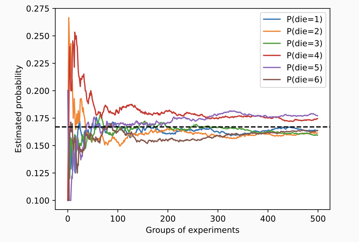
概率
from torch.distributions import multinomial

fair_probs = torch.ones([6]) / 6
multinomial.Multinomial(1, fair_probs).sample()
#每次会输出形如tensor([0., 0., 1., 0., 0., 0.])

multinomial.Multinomial(10, fair_probs).sample()
#tensor([5, 3, 2, 0, 0, 0])
向量化的采样远快于普通的 for 循环.
查阅文档
查询随机数生成模块的所有属性
print(dir(torch.distributions))

#['AbsTransform', 'AffineTransform', 'Bernoulli', 'Beta', 'Binomial', 'CatTransform', 'Categorical', 'Cauchy', 'Chi2', 'ComposeTransform', 'ContinuousBernoulli', 'CorrCholeskyTransform', 'CumulativeDistributionTransform', 'Dirichlet', 'Distribution', 'ExpTransform', 'Exponential', 'ExponentialFamily', 'FisherSnedecor', 'Gamma', 'Geometric', 'Gumbel', 'HalfCauchy', 'HalfNormal', 'Independent', 'IndependentTransform', 'Kumaraswamy', 'LKJCholesky', 'Laplace', 'LogNormal', 'LogisticNormal', 'LowRankMultivariateNormal', 'LowerCholeskyTransform', 'MixtureSameFamily', 'Multinomial', 'MultivariateNormal', 'NegativeBinomial', 'Normal', 'OneHotCategorical', 'OneHotCategoricalStraightThrough', 'Pareto', 'Poisson', 'PowerTransform', 'RelaxedBernoulli', 'RelaxedOneHotCategorical', 'ReshapeTransform', 'SigmoidTransform', 'SoftmaxTransform', 'SoftplusTransform', 'StackTransform', 'StickBreakingTransform', 'StudentT', 'TanhTransform', 'Transform', 'TransformedDistribution', 'Uniform', 'VonMises', 'Weibull', 'Wishart', '__all__', '__builtins__', '__cached__', '__doc__', '__file__', '__loader__', '__name__', '__package__', '__path__', '__spec__', 'bernoulli', 'beta', 'biject_to', 'binomial', 'categorical', 'cauchy', 'chi2', 'constraint_registry', 'constraints', 'continuous_bernoulli', 'dirichlet', 'distribution', 'exp_family', 'exponential', 'fishersnedecor', 'gamma', 'geometric', 'gumbel', 'half_cauchy', 'half_normal', 'identity_transform', 'independent', 'kl', 'kl_divergence', 'kumaraswamy', 'laplace', 'lkj_cholesky', 'log_normal', 'logistic_normal', 'lowrank_multivariate_normal', 'mixture_same_family', 'multinomial', 'multivariate_normal', 'negative_binomial', 'normal', 'one_hot_categorical', 'pareto', 'poisson', 'register_kl', 'relaxed_bernoulli', 'relaxed_categorical', 'studentT', 'transform_to', 'transformed_distribution', 'transforms', 'uniform', 'utils', 'von_mises', 'weibull', 'wishart']
使用 help:
help(torch.ones)