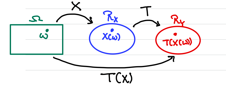
Consider a probability space . A RV and a . We can compound them to .
Technical detail: needs to be a measurable function.
So we have measurable spaces ( is the -algebra)
For all , require . Here is the preimage of .
Example
, , .
This transformation is not invertible, but preimage is well defined.
We want to know what the distribution of is.
Change of Variable Principle:
For a given , the distribution of is determined by the distribution of .
For (technically ),
For discrete case,
For continuous case, define . Then (1.1) leads to Here the p.d.f is given by .
For , .
For continuous RV, it is always .
2 Invertible Transformation
Cauchy
For such a case, , .
For ,
Meanwhile so So .
In general, if is invertible and is differentiable, the p.d.f of is given by
Log-normal
Commonly used in economics, stock market analysis, engineering, biology, etc.
, . Since , by the formula (1.2)
A noticeable fact is that, all moments of exist: However MGF doesn't exist, because So we cannot find the interval .
3 Many-to-One Transformation
Now we see a case of non-invertible function.
Chi-square on Gamma
, . For ,
i.e.
This is (see here) (or ) distribution. We can calculate the MGF
Many-to-One Transformation
Suppose of each consists of a finite or countably infinite set of points , where are differentiable. Then
Length of a Standard Gaussian Vector in
Let . , then
For (or ) with p.d.f it also has , so .
Now let , then so
4 Quantile Transformation
We know c.d.f . For , the quantile of is defined to satisfy , provided that it exists.
However, in many cases it does not exist. For example, , is not unique, and does not exist for .
To address these issues, define
Quantile Function
For , define quantile function
For ,
Inverse Transform Sampling
Let .
either discrete or continuous, then .
continuous, then .
Proof
.
Here , .
So
If continuous, inverse exists and .
For , since is strictly increasing,